Flight Simulation on the Raspberry Pi

Takeoff

A Raspberry Pi 4B with Linux can solve the equations for a real-time nonlinear aircraft simulation, including the emulation of modern aircraft flight displays.

Flight simulators range from games to airline operations, and generally, you cannot (or you are not permitted to) modify the software. Often, the code is proprietary and not accessible, or the acquisition of data used in the simulator is very costly, and the developers of these simulators are understandably protective of their software. However, for a class of simulator known as an engineering flight simulator (EFS) – used by aircraft manufacturers, avionics companies, research organizations, and universities to develop and evaluate aircraft designs and aircraft systems – it is essential to have access to the source code to modify the simulator for a range of studies.

Flight simulators have two important characteristics. First, the accuracy of the simulation (known as fidelity) should ensure that the performance and dynamics of the simulator closely matches the aircraft it simulates. For many flight simulator games, the models are simplified, reducing the fidelity to a level unacceptable in engineering applications. Second, the software must respond in real time to inputs and solve all the underlying equations at a sufficient rate (known as the frame rate), so that the perceived motion is smooth and continuous, without any noticeable lag. If the computations in simulation software are complex, the frame rate may not be sustained, and delays (latency), which further reduce fidelity, are apparent. To ameliorate this situation, a high-performance computer with a state-of-the-art graphics card may be needed to achieve the required frame rate.

Having developed real-time software for flight simulators at the universities of Southampton, Cranfield, and Sheffield; Queen Mary University (London); and the University of Newcastle (Australia), I evaluated the capabilities of the Raspberry Pi (RPi) computer with Linux to provide an acceptable EFS. Details of the software for this EFS are described in a recent textbook Flight Simulation Software: Design, Development and Testing. Wiley, 2022. The software referred to in this article is open source and can be downloaded from the Wiley Student Companion Site. The existing simulator software, which was developed for PCs and mostly written in C, ran under Linux and, for compatibility with Linux, also ran under the MSYS2 programming environment on Windows. The software for the aircraft displays was originally written in legacy OpenGL but has been rewritten for OpenGL v4 for the RPi to exploit the power of the Broadcom graphics processing unit (GPU), increasing the rendering rate of the graphics for the displays by a factor of more than 10. The performance of the RPi has enabled the PCs to be replaced with off-the-shelf RPi computers.

A Distributed Architecture

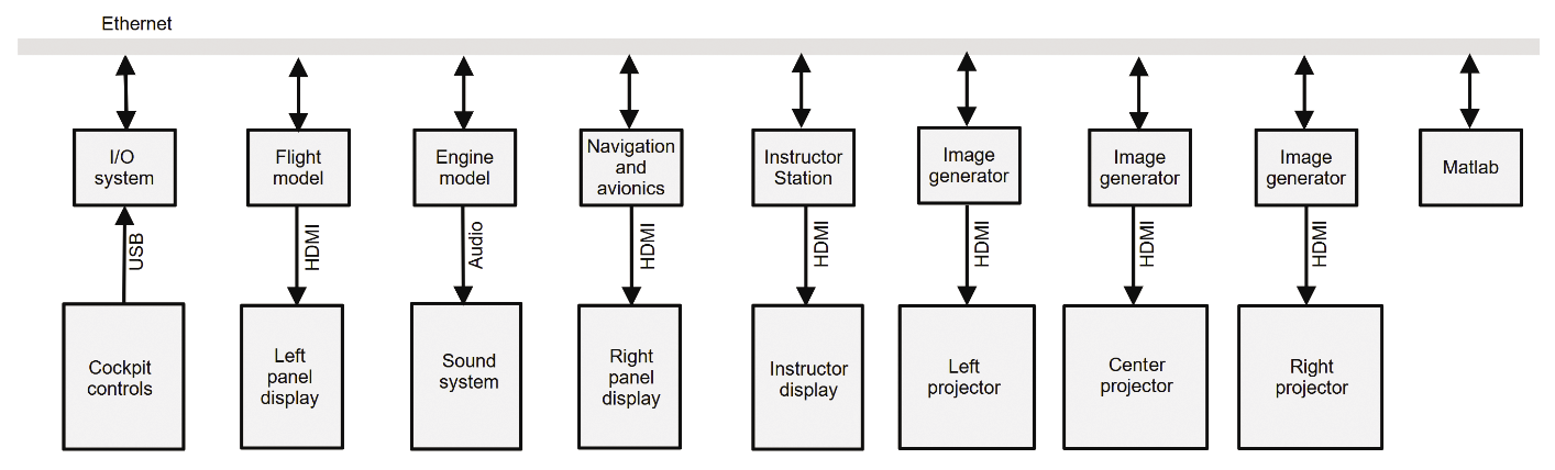
By computing a simulation on n computers, the potential increase in performance is a factor of n compared with a single computer. However, this simplification is based on two assumptions: First, the problem can be partitioned to run efficiently on n computers; second, any overhead from managing communications between the computers is negligible. The architecture of most flight simulators is particularly suited to a configuration of parallel processes. Figure 1 shows a typical organization of simulator modules, where the functions of the computers are summarized in Table 1.

Data is broadcast by modules at the start of every frame as Ethernet packets using a token-passing protocol based on the User Datagram Protocol (UDP). A computer only broadcasts a packet when it holds the token and otherwise listens for incoming UDP packets. In fact, the token is simply the arrival of a broadcast packet from the preceding node in the chain of transfers. Typically, these transfers occupy less than 2ms of the 20ms frame (Figure 2).

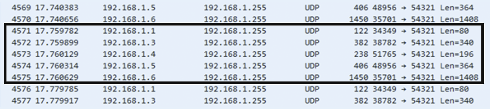
The advantage of using broadcast UDPs is that the simulator data is transmitted in five packet transfers (2,388 bytes/frame). Additionally, Ethernet provides a 32-bit checksum to ensure data integrity. Although a UDP packet transfer has no acknowledgement, with a dedicated network and a relatively low level of traffic, the data error rate is negligible.

OpenGL and GPUs

OpenGL has been used in 2D and 3D computer graphics applications since the 1990s. However, since version 3, OpenGL was repurposed to exploit the power of the GPUs found on modern graphics cards. In particular, GPUs provide fast rendering of textured triangles. In addition to the software for rendering dots, lines, and triangles, shader programs must also be provided to define how objects are rendered (the vertex shader) and how the pixels are written to a frame store (the fragment shader). To reduce the amount of detail in terms of GPU programming, a library glib was developed specifically to emulate aircraft displays that includes functions for the rendering of vectors (lines) and triangles and for applying textures to triangles. Although OpenGL does not directly support the rendering of text, standard fonts can be organized as textures, known as a texture atlas, reducing text generation to the rendering of sub-textures of a texture atlas.

Whereas objects rendered one-by-one in legacy OpenGL considerably slowed the interface between the host processor and the graphics card, with OpenGL v4, objects can be written to a cache in the host computer and transferred to the GPU as a single block when the cache needs to be flushed. For aircraft displays, this organization of caching graphics reduces the computations in the host to a minimum, enabling the parallel processing of the GPUs to maximize the rendering speed. From a programmer’s perspective, glib provides a small set of primitives to draw lines and triangles, load and render textures, load fonts and render text, and apply graphics transformations, including translation, rotation, scaling, and clipping of graphics objects, but without any explicit calls to OpenGL.

Flight Simulator Displays

Figure 3 shows the primary flight display (PFD) and the navigation flight display (NFD) produced by a Raspberry Pi 4B (RPi4B) for a Boeing 747-400. The PFD uses vectors for the sliding scales and text rendering for the digits. The rotating digits in the airspeed and altitude windows are implemented by clipping the characters to the small windows. The gray segments of the engine displays are produced offline as SVG textures and then rotated and clipped. Note the clear lines of the engine displays, which are also produced from SVG textures rather than vectors.

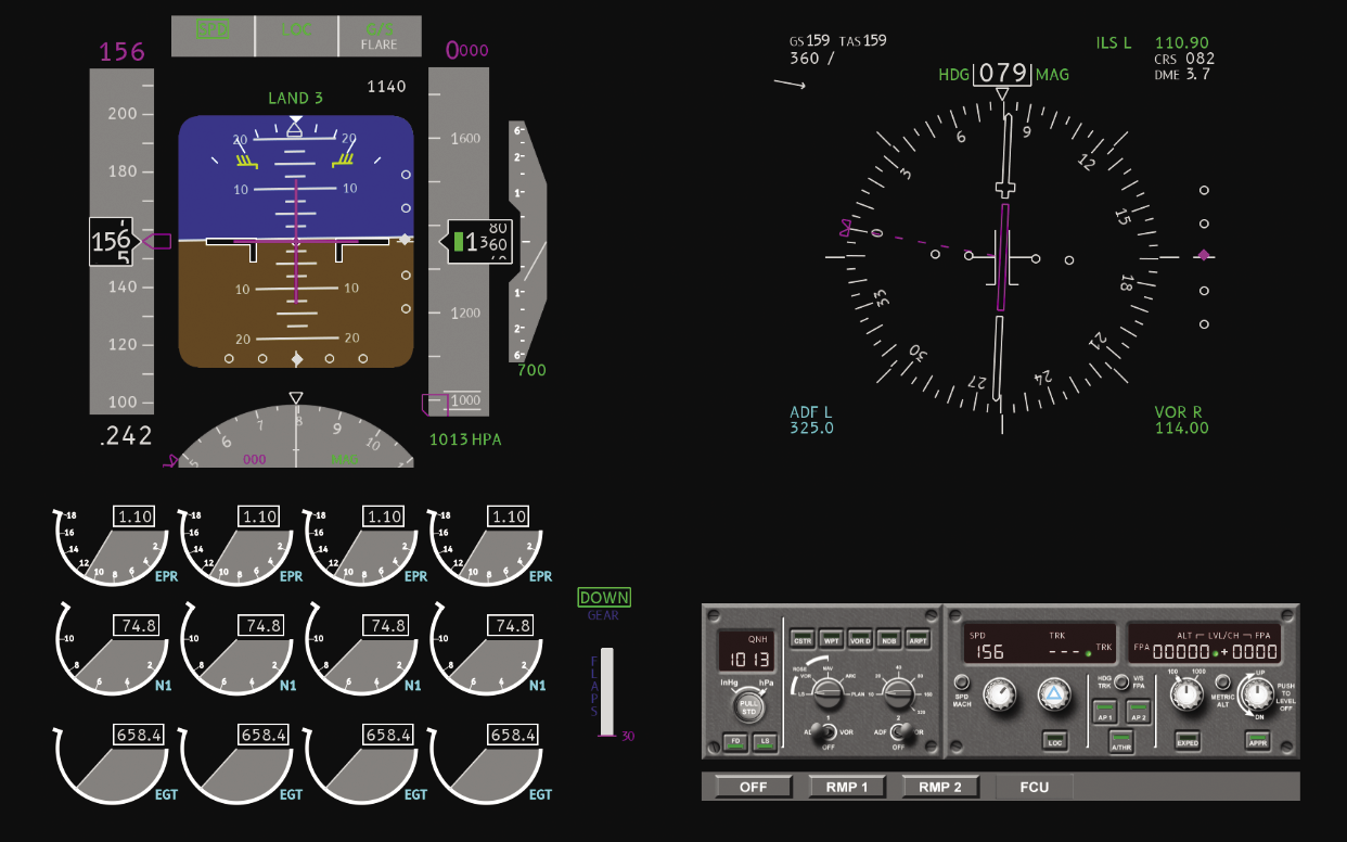
The NFD also contains vectors and text for the navigation display. The flight control unit (FCU) panel, which provides mouse or touchscreen interaction, is rendered as a texture, with character generation applied to the three small panels. The rendering of each display takes less than 3ms of the 20ms frame.

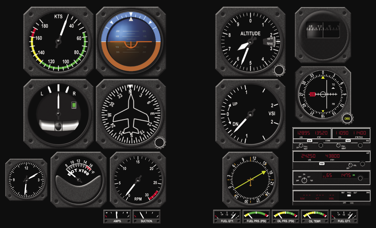
Similar methods are used to emulate the more classic displays found in light aircraft (Figure 4). The instrument bezels, static scales, and pointers are rendered as textures. The compass card is also a single texture, which is rotated in a single operation, rather than rotating all the characters and vectors of the card. The artificial horizon is rendered as a 3D sphere, which is illuminated to emphasize the curvature of the sphere, and the magnetic compass in the top right corner of the display is handled similarly.

In airline flight simulators, military simulators, and an EFS, the instructor plays an important role, setting conditions, initiating events such as an engine failure, and monitoring the activity of the flight crew. In an EFS, a further requirement is to acquire, display, and record flight data produced during testing. From the graphics perspective, these requirements imply a user interface to control and monitor simulator sessions and the display of charts and flight data. The graphics library glib, developed for aircraft displays, is also used for the instructor operating station (IOS; Figure 5).

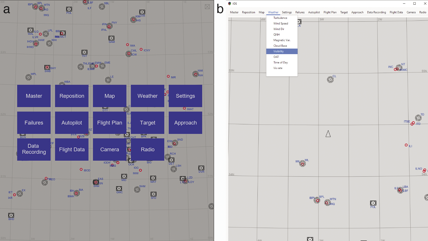
In both displays, the lines for charts and plotting are rendered as vectors, and the navigation symbols are rendered from a texture atlas by glib functions. The IOS also captures data from the other simulator computers for the plotting and recording of flight data. In this case, raw 1KB blocks of data are written to memory every frame (3MB/min) and subsequently copied to disk. The attraction of this method is that the frame rate is unaffected, the data can also be viewed off-line by a similar set of plotting tools, and the packets can be retrieved from a disk file, providing inputs to the simulator software to replay any test or exercise.

Octave and Matlab

During development of an EFS, particularly for flight control laws, sometimes it is more convenient to develop algorithms with tools like Matlab or Octave, rather than coding directly in C. Because both Matlab and Octave are interpreted languages, care is needed to ensure that any latency introduced by these packages does not affect the simulator frame rate. Although the development of detailed real-time nonlinear flight models in Matlab may be impracticable, small modules, such as automatic flight control laws can be developed and tested in Matlab, where a Matlab module acquires inputs from the simulator and generates outputs for the simulator flight controls.

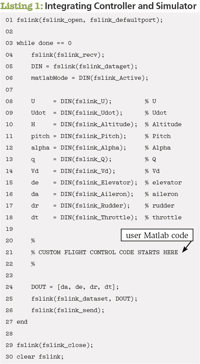
A wrapper was developed with Matlab mex functions so Matlab could read flight data from broadcast packets and transmit a packet to the simulator. The network protocol was adapted to enable Matlab to connect to, and disconnect from, the network without affecting the integrity or speed of the network protocol. The template in Listing 1 allows a controller written in Matlab to be integrated with the simulator.

Flight Simulator on a Single RPi

Having developed real-time simulator software running on five RPi computers with three displays, a further development was to combine this software for a single RPi with a single monitor (1920x1080 resolution), where the PFD is rendered on the left-hand side of the display and either the NFD or the IOS is rendered on the right-hand side, as selected by the user. To maximize reuse of the simulator software, packet passing was emulated by copying the relevant regions of memory associated with each module. Although the parallelism could be retained by treating the modules as POSIX threads, it is simpler to execute the simulator code sequentially, cycling through the modules. The main concern with this approach is that the RPi is further loaded with computations of the simulation, particularly the additional graphics rendering, compared with the multiple-processor version.

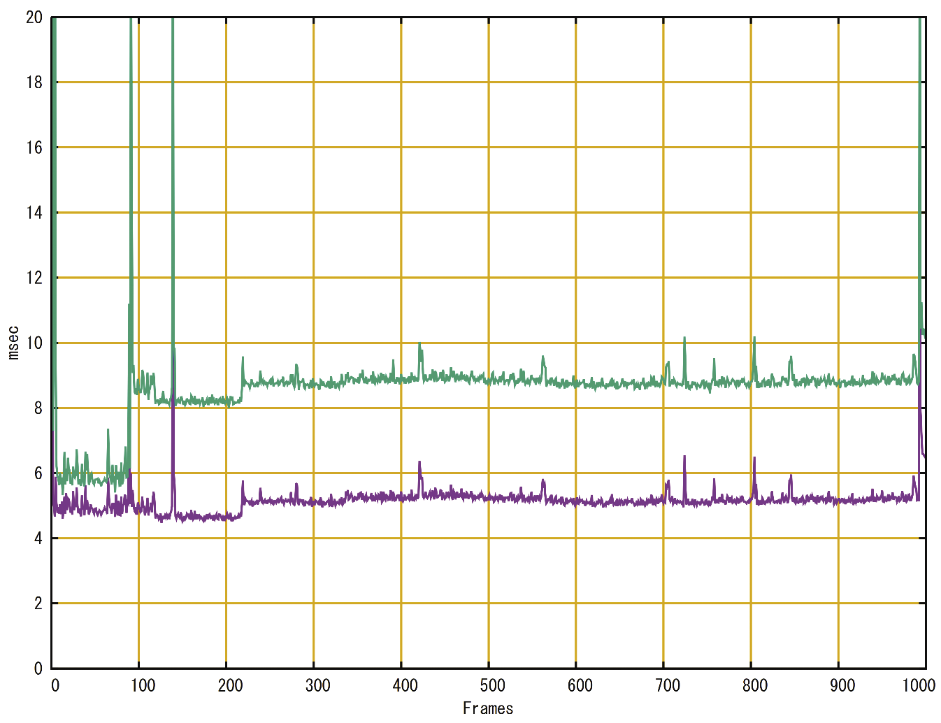
Figure 6 shows the overall frame time for the single RPi version for 1,000 frames (20s) of simulation, where the display changes several times in response to instructor actions. The lower trace shows the graphics rendering time and occupies less than 6ms/frame. The upper trace shows the overall computing time and occupies less than 10ms/frame, leaving a margin of approximately 10ms. The large excursions occurred when the simulator files were loaded at the start of the simulation and when the aircraft position was reset after 140 frames.

Offline Simulation

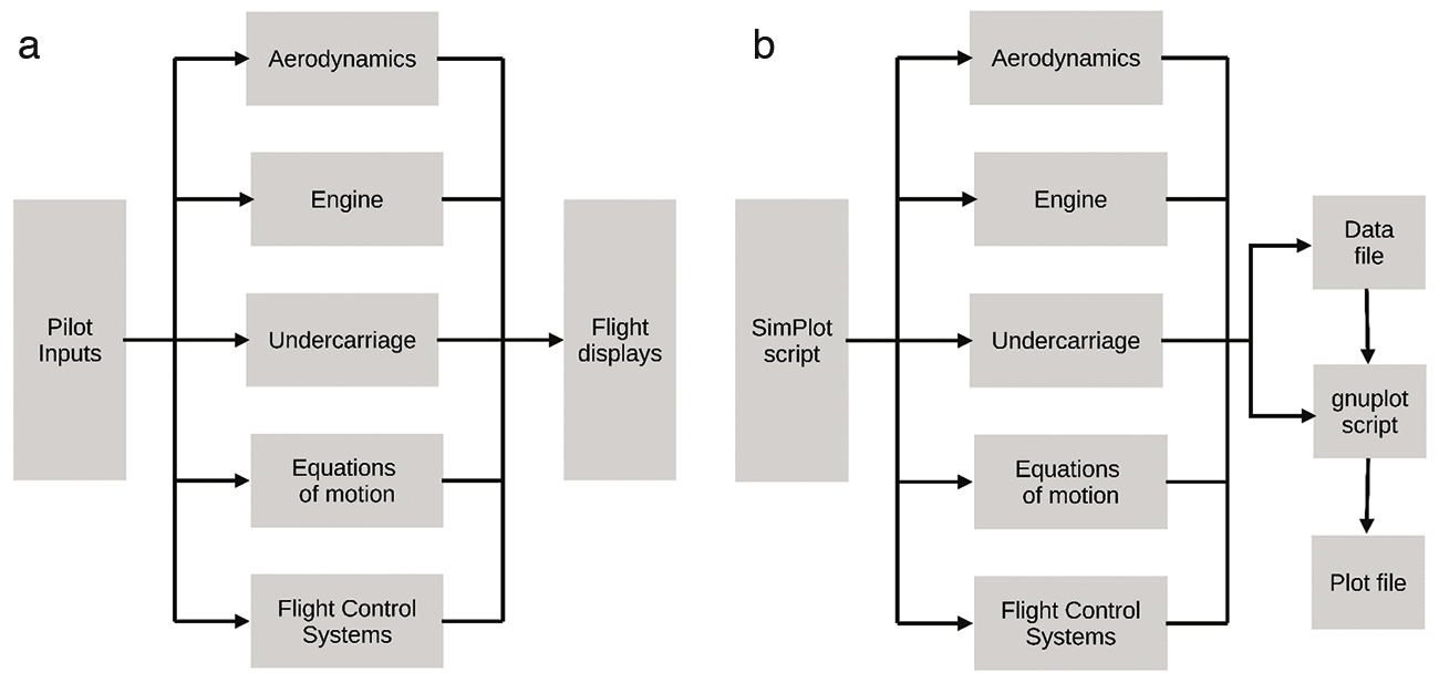
Development of prototype software can take up a considerable amount of simulator time. In this situation, access to an off-line desktop simulator, with software that is identical to the flight simulator, can provide a valuable design asset. Consider the two configurations shown in Figure 7. Two significant points can be drawn from this example. First, the main modules are identical and can be interchanged between the flight simulator and the offline simulator, and vice versa, without modification. Second, there are no real-time deadlines with an offline simulator, which can run faster than real time (e.g., simulating several hours of flight in a few minutes, typically as part of automated testing).

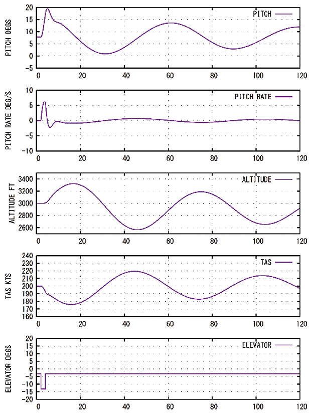
A typical output plot is shown in Figure 8. Listing 2 is the script file to run the simulation, which defines the initial conditions of the aircraft, the variables to be plotted, and the details of the plots. The autotrim command sets the aircraft in the trimmed state at the start of the exercise. The plots show the response of the aircraft to an elevator pulse input of -10° for 2s, applied after 2s. In addition to the output data, a further script is generated for gnuplot, so plots can be produced as PNG files.

Listing 2: Simulator Script

set altitude 3000 ft
set TAS 200 kts
set flaps 0.0
set gear 0.0
plot pitch degs ‑5 20
plot pitch_rate deg/s ‑10 10
plot altitude ft 2500 3500
plot elevator degs ‑20 20
time 120 secs
input elevator pulse 22 ‑10
autotrim

Visualization

Although an image generator (IG) is normally used to render the external view seen from the flight deck, for an EFS, the IG can also be used to visualize data in real time. For example, in a study of wake vortex encounters, a dedicated computer was connected to the flight simulator network to compute the flows of a wake vortex, derived from detailed vortex data. Figure 9(a) shows the wake vortices shed by an aircraft, which were implemented as billboards in the visual scene. Figure 9(b) shows the air flows and aircraft loading during a wake vortex encounter. This visualization illustrates the direction and magnitude of the air flows given by the white vectors; the loading on the wings and tail resulting from the encounter, which is color-coded; and the extremities of the vortex field shown as a red wireframe volume.

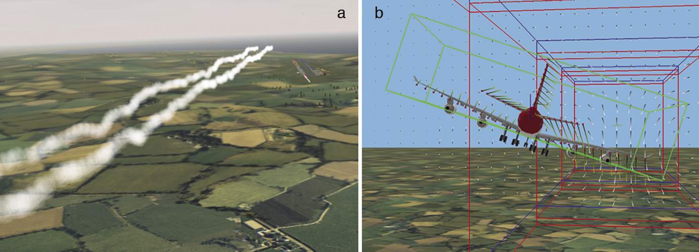
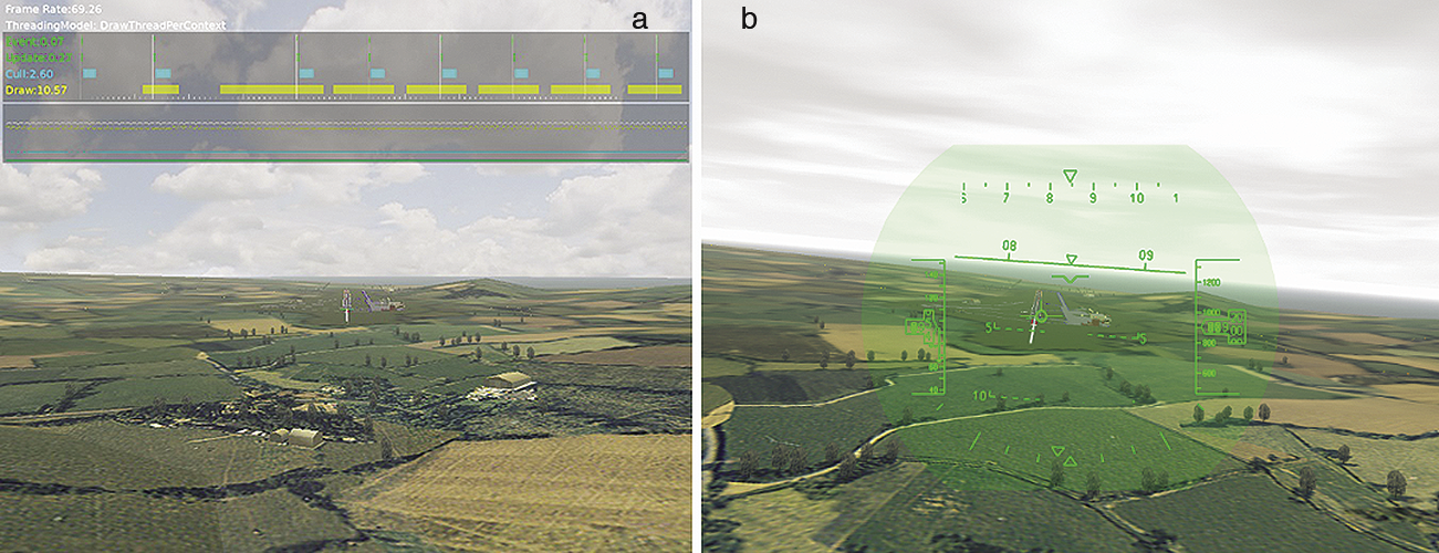
Figure 10(a) is generated by OpenSceneGraph on an RPi with an OpenFlight visual database of Bristol Lulsgate airport and achieves a frame rate of 69 frames/s (fps) for a display resolution of 1280x1024. Figure 10(b) shows a similar scene, which includes a head-up display (HUD) rendered in OpenGL as a 2D overlay on the visual scene.

Conclusions

The RPi4B with Linux is clearly capable of solving the equations for a real-time highly nonlinear simulation of a four-engine wide-body transport aircraft at 50fps, including the emulation of modern electronic flight instrument system (EFIS) displays. By providing the complete source code, the simulator modules and aircraft displays can be modified for a range of applications. With the addition of the acquisition, display, and recording of flight data during simulations, an EFS running on a single RPi can provide a particularly valuable test bed for the design and analysis of aircraft and aircraft systems. In a university, the EFS provides both a powerful facility for student projects and a totally programmable simulation environment for research in aircraft design and system validation.